Ask an LLM how sure it is about something and when it answers you, it gives you a number based on vibes. “I’m about 90% confident” comes out of the same next-token machinery as everything else it says. The 90 is a word choice, not a measurement, and it will say it just as warmly about something it made up.
Watch it happen. Give an LLM the last few days of weather and ask it to forecast tomorrow’s:
{
  "09/27/2026": 59, // date and temp in Fahrenheit
  "09/26/2026": 57,
  "09/25/2026": 64,
  "09/24/2026": 63
}
The obvious thing is to ask for a single number, and while we’re at it, ask how sure it is:
llm.generate(
  prompt: "Given the last 4 days of temps, forecast tomorrow: " + weather,
  schema: {
    "date": string,
    "temperature": number,
    "confidence": string
  }
)

// => { "date": "09/28/2026", "temperature": 60, "confidence": "about 90%" }
Sixty degrees, about 90% confident. Sounds great. Now ask where the 90 came from. Nothing in that call gave the model a way to measure how sure it is; it produced “about 90%” the same way it produced “60”, by predicting what a confident forecaster would say next. Its real uncertainty comes from two places: how much data and prior knowledge it has, called epistemic uncertainty, and the plain unpredictability of the future, called aleatoric uncertainty. The first shrinks as we collect more history; the second never goes away. Suppose we had only one day of history, and it was a freak hot day. The model should be far less sure about tomorrow, and “about 90%” would come out just the same.
The language of uncertainty is the probability distribution. Instead of asking for one temperature, take the full range ever recorded in the area, split it into buckets, and ask the model to put a probability on each. Those probabilities sum to 1 and together form a distribution over tomorrow’s temperature. A confident model piles most of its probability into one or two buckets; an uncertain one spreads it out.
// one bucket per 10°F, covering every temp on record
llm.generate(
  prompt: "Yesterday was 95°F. Forecast tomorrow's high.",
  schema: {
    "30-39": probability,
    ...
    "100-109": probability
  }
)

// => { "50-59": 0.20, "60-69": 0.30,
//      "70-79": 0.22, "80-89": 0.15, ... }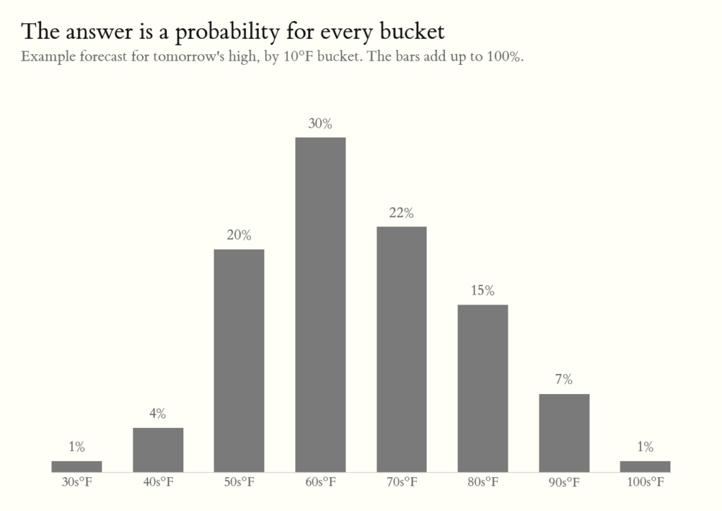
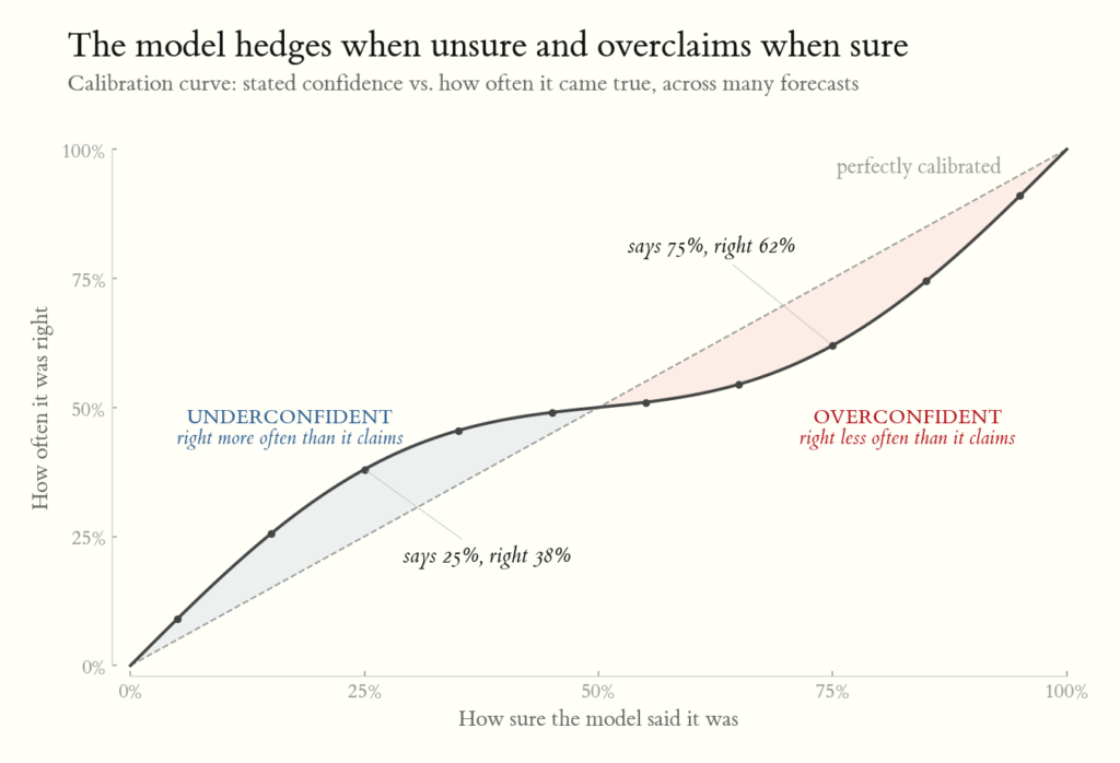
A forecast distribution is only a claim about the world. To check it we need the real distribution: across all the days the model made this same forecast, how often tomorrow’s high actually landed in each bucket. We aren’t grading whether the model got tomorrow right. It can’t be perfectly right, because part of the future is simply unpredictable. We’re grading whether it’s honest about how sure it is. A calibrated model’s claims line up with the outcomes: of all the days it gave 60-69°F a 30% chance, about 30% landed there. An overconfident model piles probability into a couple of buckets while outcomes scatter wider. An underconfident model spreads its bets while reality clusters tightly. A calibrated model will still be wrong plenty of the time, but when it says it’s more sure of one outcome than another, you can trust that number.
So how does RLCD teach a model to do this? The same way a forecaster learns: by checking forecasts against what happened. The model makes its forecast, then tries a handful of slightly different versions of it: one a little more sure of the 60s, one leaning a little warmer, and so on. The next day the real high comes in the 70s. Each version is scored by how much chance it gave the 70s; more chance on what actually happened means a higher score. The model shifts toward the versions that beat the average and away from the ones that fell short, then repeats this over thousands of questions.
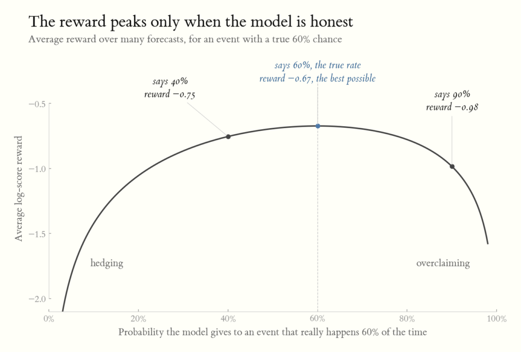
The clever part is the score itself. A model that always acts sure gets punished hard whenever it’s wrong. A model that always hedges never scores well, even when it’s right. The only way to maximize the score over many questions is to say exactly how sure it should be: if something happens 60% of the time, the best score comes from saying 60%, not 40% and not 90%. So the model isn’t just learning to be right; it’s learning to be honest about how likely it is to be right. Laya, trained this way, reports that its stated confidence is off by about 6 points on average.
Once a probability is calibrated, you can do arithmetic with it instead of eyeballing it. An uncalibrated “90% confident” from a model is a word choice. A calibrated 90% is a number you can wire straight into expected-value math.
To see this with a real decision instead of a temperature bucket, imagine JEV as the forecaster. Give it a stock’s recent price action, options flow, and news, and ask for a calibrated distribution over where tomorrow’s close lands.
from typesafe_sdk import Choice, TypeSafeClient

client = TypeSafeClient()

response = client.system_one(
  state="NVDA closed today at $180. Price action, options flow, and news over the last 5 trading days.",
  questions={
    "closing_range": Choice(
      instructions="What range will NVDA's closing price fall in tomorrow?",
      criteria={
        "165-170": "Closes between $165 and $170",
        "170-175": "Closes between $170 and $175",
        "175-180": "Closes between $175 and $180",
        "180-185": "Closes between $180 and $185",
        "185-190": "Closes between $185 and $190",
        "190-195": "Closes between $190 and $195",
        "195-200": "Closes between $195 and $200",
      },
    ),
  },
)

probabilities = response.answers["closing_range"].probabilities
# => {"165-170": 0.05, "170-175": 0.13, "175-180": 0.20,
#     "180-185": 0.28, "185-190": 0.20, "190-195": 0.09, "195-200": 0.05}
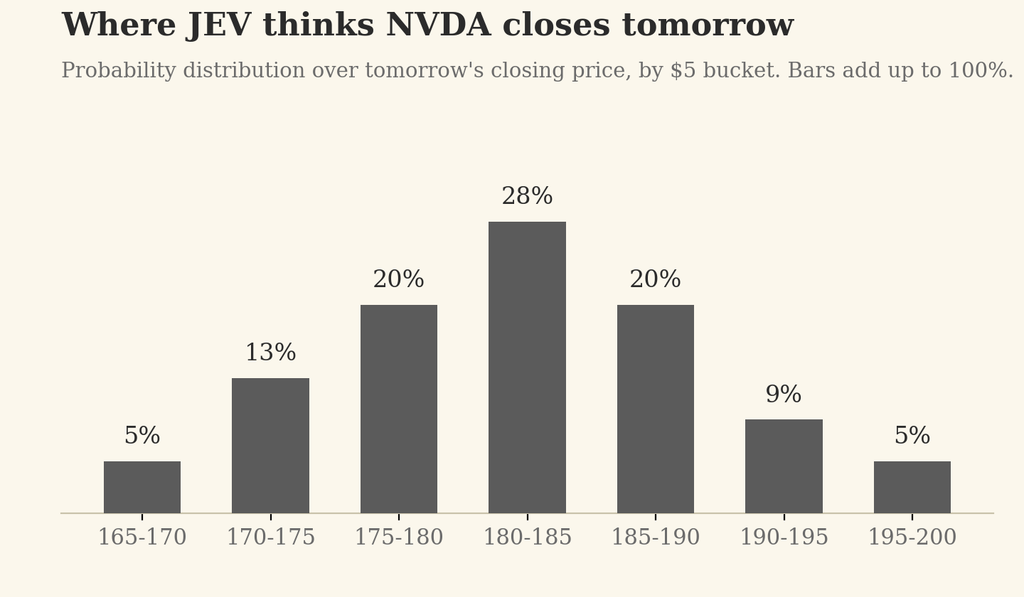
NVDA closed at $180, so “up” means landing in a bucket above that price. Summing the probability on those buckets collapses the whole distribution into the one number Kelly needs:
p = sum(probabilities[b] for b in ["180-185", "185-190", "190-195", "195-200"])
# => 0.62
That 0.62 means something only if JEV was trained the way RLCD trains; otherwise it’s a number that sounds confident. If it is calibrated, we can feed it straight into the Kelly criterion, which turns “62% chance it’s up” into “how much of the account to risk, if anything”:
def kelly_fraction(p, b=1):
  return p - (1 - p) / b

kelly_fraction(0.62)
# => 0.24   →  buy, sized at 24% of bankroll

kelly_fraction(0.52)
# => 0.04   →  buy, sized at 4% of bankroll (barely worth it)

kelly_fraction(0.48)
# => -0.04  →  negative Kelly: don't buy, JEV's own number says there's no edge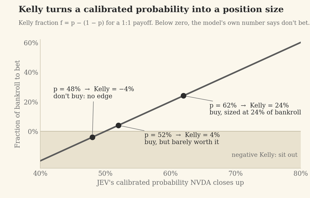
The calibrated probability decides whether the pick is worth acting on at all, and how hard to lean on it. Take away the calibration and you have no principled way to size the bet, or to know when to sit out.
So I ran it for real. I gave JEV the last eight sessions of NVDA’s actual OHLCV (Friday’s close was $225.07), added open-ended tail buckets so the ranges cover every possible close, and asked the same question:
The probabilities sum to exactly 1.0, every run, and the answer barely moves between runs. But look at the shape. JEV put 95% on a single $5 bucket sitting on Friday’s close. NVDA’s realized daily volatility over the last 50 sessions is 2.46%, about $5.54 a day, so that bucket deserves something like 30%. Here is JEV’s distribution next to the empirical one, which is just the last 49 daily returns applied to Friday’s close:
| Bucket | JEV | Empirical (last 49 days) | Lognormal fit |
|---|---|---|---|
| below 210 | 0% | 0% | 0% |
| 210-215 | 0% | 4% | 2% |
| 215-220 | 0% | 12% | 13% |
| 220-225 | 5% | 31% | 30% |
| 225-230 | 95% | 27% | 33% |
| 230-235 | 0% | 24% | 17% |
| 235-240 | 0% | 0% | 4% |
| 240-245 | 0% | 2% | 1% |
| 245 and up | 0% | 0% | 0% |
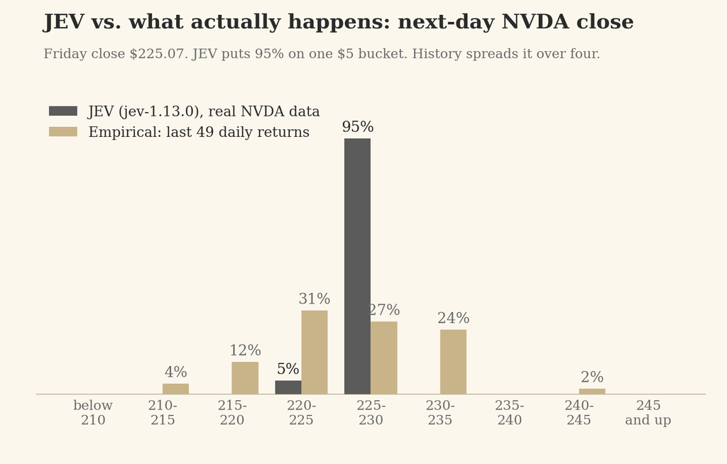
That is the overconfident shape from the calibration chart above: probability piled into one bucket while the outcomes scatter across four. Push it through the same math and it says p_up = 0.95 and a Kelly fraction of 0.90, so bet nine tenths of the bankroll on what history says is roughly a 53/47 coin. The number sounds confident, and for this question it is not calibrated. Which is the point. The calibration RLCD buys you covers the distribution the model was trained on, and next-day NVDA closes evidently aren’t in it. You can’t fine-tune JEV to your domain; it’s a closed model behind an API. But you can take an open-source model like Laya and post-train it with RLCD on your own outcomes, the same forecaster-checks-the-weather loop, until its numbers are calibrated for the question you actually ask. A decision model earns the right to be wired into Kelly one domain at a time, and you check whether it has earned it the same way you check a weather forecaster: score it against what actually happened.
In short, calibration is what turns the model’s confidence from a vibe into a control signal. That is what RLCD is really training: not the answer, but the honesty of the number attached to it. A model that says 60% and is right 60% of the time can be wired into expected-value math, into Kelly, into any downstream decision that needs to know how far to trust it. A model that says 95% and is right 30% of the time can’t be wired into anything; you’re back to eyeballing. And as the NVDA run shows, that honesty reaches only as far as the training data, which is why being able to run the loop yourself on an open model matters as much as the loop itself.