Your backlog is sitting idle waiting to get worked on, and it could be showing up pre-baked, ready for verification.
openclaw polls my Linear backlog every 30 minutes for tickets tagged openclaw. For each ticket, it creates a session and a git worktree of our our codebase if one doesn’t already exist, and the cron agent decides whether the subsession needs an update based on the contents of the current ticket.
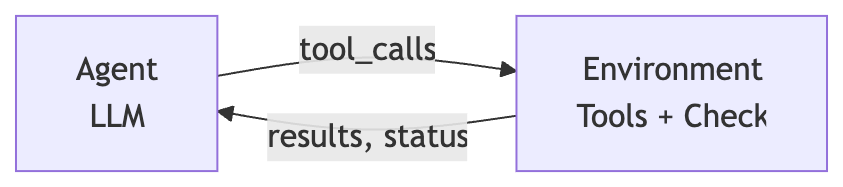
flowchart LR
    L[Linear] -->|ticket info| O[Cron Orchestrator]
    O -->|create or update| S1[Sub-agent session: ticket A]
    O -->|create or update| S2[Sub-agent session: ticket B]
    O -->|create or update| S3[Sub-agent session: ticket C]

    classDef default fill:#fff,stroke:#333,stroke-width:1px,color:#000
That’s the whole system. Once openclaw is up and running with github and linear access, a 15–45 minute session is enough to teach it a workflow like this.
Poll vs Webhook
The natural way to build a Linear agent is event-based: a webhook hitting an internal endpoint with auth. Drop the real-time requirement and the webhook drops with it. Polling needs no route, no signed payload, no inbound auth. Just a Linear API key.
Why 30 Minutes, Not Real-Time
The 30-minute loop sets a different expectation around the interaction. Linear replies were never expected to be real-time anyway, so the slower cadence just matches the surface you’re already collaborating on. Slowing down the interaction is what makes higher throughput possible.
A Form Factor for Ralph-Loop and Autoresearch Tasks
You can assign openclaw a ralph-loop or autoresearch task and collaborate on it directly in Linear. This is basically how open source software has been developed forever. async, with no expectation of an immediate response. The new part is that the dev on the other end is a openclaw sub agent session instead of a person.
Go With the Flow
For the important but not-urgent work, lean into the async. My current loop is already a plate-spinning act of agents. I have now moved this into one of my plates to spin. I can drop this plate without caring because its my backlog. The async nature of these tasks means they don’t need my immediate attention. What has changed is that I can make small incremental progress on them as a part of my normal dev routine instead of them idling collecting dust. Given that the nature of this work is such that it normally rots, even having one of these land is a win for me.
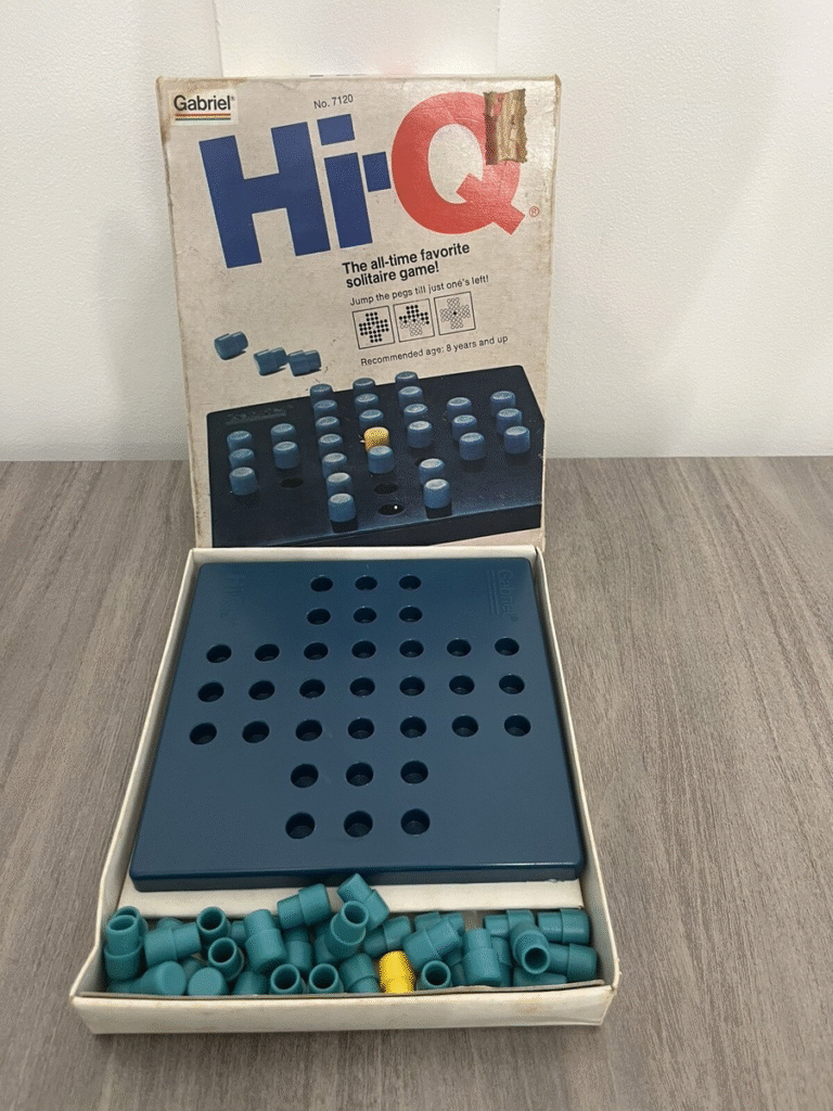
On a snowy day at my parents’ house, I was passing time with family and reading a blog post about planner programming when my grandmother invited me to play Othello at her apartment. While getting the game out of her cabinet, I noticed a box for Hi-Q. I owned this game as a child and had played it to the point where I could reliably win with one peg left every time. To my disappointment, I could only get down to 4 pegs when I tried again now. While my Hi-Q skills had atrophied, my programming skills have improved considerably—I wondered if I could find an optimal solution using Picat. I couldn’t. But I did find a way to solve it with deep learning.
Attempt 1: Constraint-Based Approaches
I installed Picat and vibe-coded some scripts to find a sequence of moves leading to one peg in the center using the planning module. The scripts ran indefinitely without producing output—the search space was simply too large.
I’m the author of a MiniZinc MCP server connected to my Claude account. Since planners are essentially a DSL on top of constraints, it seemed like a constraint-based solution should work. But Claude’s solutions also timed out.
Looking for hints, I found a paper on Integer Programming Based Algorithms for Peg Solitaire Problems. The key insight: the search space is large enough that you need sophisticated pruning methods. I could have fed this paper to Claude and been done with it, but I wanted a solution I actually understood. The integer programming approach would have been another black box. This motivated my pivot to deep learning—the loss function was intuitive, and I suspected a neural network would naturally learn to prune the search space.
Attempt 2: PPO
My previous experience with reinforcement learning was using Proximal Policy Optimization in PyTorch to solve simple Gym environments like CartPole and LunarLander. I vibe-coded a Gym environment for Hi-Q and a basic PPO network, then trained for 100k timesteps. The resulting policy reliably got down to 4 pegs. Not bad!
But the policy would converge on a solution and refuse to deviate—it was stuck in local maxima. When I analyzed the model’s behavior, it was playing the exact same 30 moves every single game, ending with two pegs that couldn’t jump each other. The +1 reward per move meant it had found a local optimum: make 30 valid moves and get stuck (+28 total reward) was good enough that it never explored further.
Attempt 3: Breaking Out of Local Maxima
Claude proposed four approaches to escape the local optimum. I tested them in parallel:
Remove per-move reward — Only reward at game end based on remaining pegs. Result: Didn’t help.
Progressive reward shaping — Exponential scaling where fewer remaining pegs = much higher reward. Result: Marginal improvement.
Higher exploration — Increased entropy coefficient from 0.01 to 0.05. Result: Didn’t help.
Curriculum learning — Start the agent on easier board states (fewer pegs) and gradually increase difficulty. Result: Significant improvement!
Only curriculum learning significantly decreased loss. After 1 million timesteps with curriculum learning, I got down to 2 pegs—but still couldn’t solve it completely.
Attempt 4: AlphaZero
The neural network needed to see examples of winning solutions to converge on one. I introduced the AlphaZero architecture, which combines neural networks with Monte Carlo Tree Search. MCTS runs simulations of possible move sequences, giving the agent the ability to plan ahead and occasionally stumble onto winning games during training.
Two changes made the difference:
MCTS depth became the most important hyperparameter—more simulations meant better planning and faster convergence
Full-board mixing—even during curriculum learning, I mixed in 20% full-board games so the model always trained on the actual problem
I fired off a 6-hour training job on an H100 and went to my family Christmas party. When I woke up, Santa had delivered an optimal solution to Hi-Q.
Reflections
The integer programming paper solved this in 15 minutes on a 2001 laptop CPU. Mine took 6+ hours on a 2025 H100. Hardly an improvement in efficiency! But I learned about curriculum learning, and I ended up with an artifact I actually understand—something I wouldn’t have gotten from the integer programming route, even with vibe coding.
This project taught me that vibe coding lets me punch above my weight class with neural network architectures. For one-off projects, it’s great: I can vibe-code slop, and as long as my network converges on something useful, that’s all that matters. I’m skeptical this strategy scales to more sophisticated projects—there’s a lot of plumbing and failure modes in deep learning. But for off-the-shelf algorithms in PyTorch, Claude Code acted as faster arms and legs to execute on my ideas and test hypotheses.
Static binaries solve distribution, but configuration files break the model. Now you’re distributing two separate artifacts, creating version mismatches and every new deployment is an opportunity for human error.
With nix, you can bundle your configuration with your binaries using a wrapper script. nix can take care of distribution of the configuration, and making sure that it shows up at the right place, and your binary references it by using nix store paths.
The flake references ./stdout.yml at build time, copying it into the Nix store. The generated wrapper script contains the full store paths for both the Vector binary and config file. When you run nix run <target>, you’re executing a closure where the binary and config are guaranteed to match. They share the same derivation hash. If either changes, the hash changes, forcing a rebuild of the entire bundle. The person deploying this doesn’t think about config files. They run one command. The correct configuration is already there.
You can use validation functions as a tool to steer coding agents and data processing agents automatically, instead of manually copy pasting outputs or prompting. You can use this to parallelize common tasks in agentic programming, and eliminate bottlenecks on your agentic coding workflows.
The Standard Agent Loop
The industry consensus on a agentic loop looks something like this
msg = []
while True:
    msg.append(input())
    while True:
        output, tool_calls = prompt_llm(msg)
        msg.append(output)
        print("Agent: ", output)
        if tool_calls:
            msg.extend([
              handle_tool_call(tc)
              for tc in tool_calls
            ])
The Problem: Manual Verification
Agents operating on this premise trap you in a tedious cycle:
Agent makes a change
Manually run tests
Paste the output back into the agent
Repeat
While this workflow might feel productive you might start to feel bottlenecked by your ability to copy paste test outputs from window to agent time and time again. To automate this, get the agent to run the tests for you and feed the results of this test back into its context window. By automating this, you can free up your attention by running this in the background, and have confidence of reaching a stable state code wise.
Naive Solution: Bro, Just Prompt Harder
fix my failing test and verify your fix by running pytest
Steering the agent via a prompt is an okay way to implement this control flow. You are handing off the control flow to token output generation so that will make your control flow probabilistic in nature and subject to all of the fun consequences of that property. One example of a failure mode here is sometimes agents will just give up after so many tries of failing tests, instead of trying a different approach.
Control for Hallucination with Deterministic Validators
introducing validation directly into the agent loop feeds back validation context into the agent so that it does not complete its loop until the goals are met.
 msg = []
 while True:
     msg.append(input())
     while True:
         output, tool_calls = prompt_llm(msg)
         msg.append(output)
         print("Agent: ", output)
         if tool_calls:
             msg.extend([
               handle_tool_call(tc)
               for tc in tool_calls
             ])
+        complete, output = check_completed()
+        msg.append(output)
+        if complete:
+          break
When an agent is ready to submit a completed task, the check_completed() function runs a verification command (like npm run test) or executes any validator that determines task completion. When the task remains incomplete, the validation output enters the message history, creating an automatic feedback loop.
flowchart LR
    Agent -->|mutation with tools| Environment
    Environment -->|observation with validators| Agent
Why This Works
This approach gives the agent grounded, controlled access to environment state. Agents possess tools to inspect the environment, but prompt-based steering proves unreliable. Agents grow lazy, confused, or prematurely declare success. Embedding environment state validation directly into control flow ensures the agent continues until either:
The task is genuinely complete, or
The token budget is exhausted
Critically, check_completed() validates the actual state resulting from the agent’s actions on the environment, not merely what the agent thinks it accomplished.
Implementation: Mini Agent Action
Mini Agent Action adapts Mini SWE Agent to implement this control flow. Install it with pip and run an agent with a bash tool that loops until task completion:
pip install mini-agent-action
mini-agent-action --exec "python test.py" \
                  --task "fix this test, you can see it fail with python test.py. you will be validated against that cmd" \
                  --debug
This sort of agent is very useful to have listening to your PR branches. When you push a commit with broken tests, instead of intervening, you can task switch and wait for this agent to come up with a solution to your test failure. Mini SWE Agent claims a 70% score on SWE bench without having this level of control on its outputs, and even if the agent doesn’t complete the task correctly, it will often be close enough to the correct answer that I am able to use part of its outputs in the final implementation. The agent creates a pull request on the feature branch, so I can choose to just merge, or close the pull request if I’m not happy with the results.
A system like this is proactively having agents fix your code, instead of having a programmer reactively prompting agents to intervene, while maintaining human ownership over the results.
Implementation: Data Transformation
Consider this common scenario: you receive JSON data that must conform to a specific schema. You could manually write transformation logic, but this approach fails at scale. Each new JSON structure requires custom transformation code—an unsustainable workload when handling diverse inputs.
Agents solve this by generating valid transformation code at runtime. Add a validation function to your agent loop that checks whether the transformed output matches your target schema. When validation fails, the agent reruns with debug information until it produces valid output.
flowchart TD
    A[Input JSON] --> B[Generate Python code<br/>to transform data]
    B --> C{Output matches<br/>target schema?}
    C -->|No| B
    C -->|Yes| E[Return valid JSON]

    classDef default fill:#fff,stroke:#333,stroke-width:1px,color:#000
    classDef decision fill:#f5f5f5,stroke:#333,stroke-width:1px,color:#000
    class C decision
This approach has limitations. Agents sometimes satisfy validation by emitting minimal, empty JSON documents. You may need multiple runs to get acceptable results. Still, this requires far less effort than writing custom transformations for each incoming schema.
Conclusion
Integrating automated validation into your agent’s control flow eliminates manual intervention and creates an autonomous system.
I read a blog post on how Many Hard Leetcode Problems are Easy Constraint Problems and was pleasantly surprised at how approachable MiniZinc was compared to other solver software I have been exposed to, and the examples given helped me to understand how to apply it to a domain I was already familiar with. I have always wanted to be able to get more familiar with using constraint satisfaction as a way to solve problems, so I decided to create a solver to help optimize storage space for Minecraft using constraint satisfaction to help learn how to use this tool. I will outline my thought process and how I reached the solution I came up with.
Game Mechanics
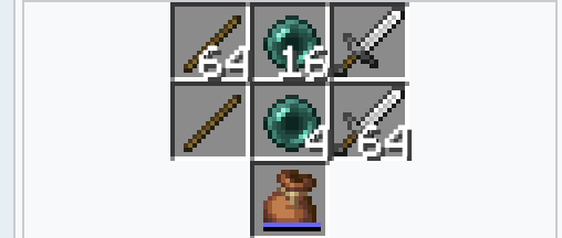
In Minecraft, your player inventory is limited. You have 27 inventory slots, 9 hotbar slots, 4 armor slots, 4 temporary crafting slots, 1 offhand slot, 1 temporary slot for the result of crafting, and you can hold 1 item in your cursor (thanks charcircuit).
Each slot can either contain a single item, a small stack of 16, or a full stack of 64 items, depending on the item.
Often when adventuring, you will come across many rare and powerful items and accumulate many items in your inventory slots, but they may be stacks of items that are not at maximum capacity for that inventory slot. Once your inventory is full, you cannot pick up new items. Using bundles, you can consolidate your inventory and pick up more items.
A bundle is an item that can store up to a stack’s worth of mixed item types within itself in a single inventory slot. Items can be individually selected and taken out of the bundle via the inventory menu.
Item stack sizes (top row) and the number of bundle slots they take up (middle row). Sticks stack to 64, so they take up one bundle slot; ender pearls stack to 16, so they take up four; and swords do not stack, so they take up the whole bundle. So, for instance, a bundle may have 32 sticks and 8 ender pearls inside, which take up a total of (32×1)+(8×4)=64 bundle slots.
Creating an Optimizer
Using the MiniZinc Playground, we can model our player’s inventory and the constraints such that we free up the maximum number of inventory slots. That way, our player can pick up the most new items!
First, let’s create an inventory and let’s only focus on items that have full stacks. We can maximize our free inventory slots for this case, and then we will progressively make our way toward supporting all of the item types.
array[int] of int: inventory = [
  % fullstack of dirt
  64,
  % half of a fullstack of wood
  32,
  % half stack of a fullstack of  wool
  32,
  % quarter of fullstack of sticks
  16,
  % quarter of a fulstack of carrots
  16
];
If our optimizer was working, it would select three slots of our inventory to go in the bundle to maximize our free inventory space. We can model inventory selection by creating another array of integers of either 0 or 1, with 1 representing a selected slot in our inventory and 0 representing an unselected slot.
int: n = length(inventory);
array[1..n] of var 0..1: selected;
Once we have this array representing our selected slots, we can maximize the sum of our array in order to select the most slots possible.
solve maximize sum(i in 1..n)(selected[i]);
The full code now will look like this
% Use this editor as a MiniZinc scratch book
array[int] of int: inventory = [
  % fullstack of dirt
  64,
  % half of a fullstack of wood
  32,
  % half stack of a fullstack of  wool
  32,
  % quarter of fullstack of sticks
  16,
  % quarter of a fulstack of carrots
  16
];

int: n = length(inventory);
array[1..n] of var 0..1: selected;

solve maximize sum(i in 1..n)(selected[i]);
Our solver found the solution selected = [1, 1, 1, 1, 1]; to maximize our selected slots in our inventory, which means it selected every slot. This makes sense because we did not constrain it in any way. Let’s add some constraints so we can now make better-informed selections.
The constraint we are exceeding is our bundle capacity. If we include our bundle capacity in our model and constrain our selections to include only inventory items that do not exceed the bundle capacity, we can find a valid solution.
If we add this constraint to our model and run it again, we can see that it now only selects three inventory slots, and it selects slots that do not exceed the capacity of our bundle.
Great! Our initial model works for items that all stack to 64, but Minecraft has items with different maximum stack sizes. As mentioned earlier:
Items that stack to 64 (like dirt, sticks) take up 1 bundle slot per item
Items that stack to 16 (like ender pearls, snowballs) take up 4 bundle slots per item
Unstackable items (like tools, armor) take up 64 bundle slots (the entire bundle)
To handle this in our model, we need to represent each item’s bundle cost accurately. We’ll use a scaled representation to avoid decimal arithmetic:
int: units = 16 * 64;  % Total bundle capacity (1024 units)
int: fullstack = 1 * 16;  % Cost per fullstack item (16 units per item)
int: smallstack = 1 * 64;  % Cost per smallstack item (64 units per item)
int: unstackable = 16 * 64 + 1;  % Cost exceeds capacity (1025 units)
Why scale by 16? This gives us clean integer values:
1 dirt item = 16 units (1 bundle slot × 16)
1 ender pearl = 64 units (4 bundle slots × 16)
Total capacity = 1024 units (64 bundle slots × 16)
Now we can model a more realistic inventory:
array[int] of int: inventory = [
  % full stack of 64 dirt (takes entire bundle)
  64 * fullstack,  % 64 × 16 = 1024 units

  % full stack of 16 ender pearls (takes entire bundle)
  16 * smallstack,  % 16 × 64 = 1024 units

  % 1 pickaxe (can't fit with anything else)
  unstackable,  % 1025 units

  % half stack of 32 dirt (half a bundle)
  32 * fullstack,  % 32 × 16 = 512 units

  % half stack of 8 ender pearls (half a bundle)
  8 * smallstack,  % 8 × 64 = 512 units
];
and the rest of the model remains the same
int: n = length(inventory);
array[1..n] of var 0..1: selected;

constraint sum(i in 1..n)(selected[i] * inventory[i]) <= units;
solve maximize sum(i in 1..n)(selected[i]);
the full example:
int: units = 16 * 64;
int: fullstack = 1 * 16;
int: smallstack = 1 * 64;
int: unstackable = 16 * 64 + 1;

array[int] of int: inventory = [
  % stack of dirt
  64 * fullstack,
  % stack of ender pearls
  16 * smallstack,
  % pickaxe
  unstackable,
  % half stacks, should select these to maximize inventory space
  32 * fullstack,
  8 * smallstack,
];

int: n = length(inventory);
array[1..n] of var 0..1: selected;

constraint sum(i in 1..n)(selected[i] * inventory[i]) <= units;
solve maximize sum(i in 1..n)(selected[i]);
When we run this on the playground, we can see that it selects the last two slots, which correctly selects the maximum number of mixed items to store in a bundle.
Using MiniZinc, we can represent our problem declaratively, making it easy to extend and modify as needed. If game mechanics change or we want to support other storage systems like shulker boxes, we can simply update our constraints. This project was an enjoyable introduction to constraint satisfaction problems, and the MiniZinc Playground made it accessible without requiring any local setup.